


Abstract
In this work, we use muon bundles, which are formed in extensive air showers and detected at the ground level, as a tool for searching for anisotropy in high-energy cosmic rays. Such choice is explained by the penetrating ability of muons that allows them to retain the direction of primary particles with good accuracy. In 2012–2022, we performed long-term muon-bundle detection with the coordinate-tracking detector DECOR, which is a part of the Experimental Complex NEVOD (MEPhI, Moscow). To search for cosmic-ray anisotropy, muon bundles arriving at zenith angles in the range from 15° to 75° in the local coordinate system are used. During the entire period of data taking, about 14 million of such events have been accumulated. In this paper, we describe some methods developed in the Experimental Complex NEVOD and implemented in our research, including: the method for compensating for the influence of meteorological conditions on the intensity of muon bundles at the Earth's surface, the method for accounting for the design features of the detector and the inhomogeneity of the detection efficiency for different directions, as well as the method for estimating the primary energies of cosmic rays. Here we present the results of the search for the dipole anisotropy of cosmic rays with energies in the PeV region and also compare them with the results obtained at other scientific facilities.
Export citation and abstract BibTeX RIS

Original content from this work may be used under the terms of the Creative Commons Attribution 4.0 licence. Any further distribution of this work must maintain attribution to the author(s) and the title of the work, journal citation and DOI.
1. Introduction
Cosmic-ray (CR) anisotropy is usually defined as the relative deviation from the assumed isotropic flux. The study of CR anisotropy on the Earth's surface is a very complicated problem that holds a lot of puzzles. The phenomenon of CR anisotropy is associated with the distribution of the CR sources on the celestial sphere, as well as with the interaction of CRs with matter and fields in the interstellar space.
An uneven distribution of CR sources and magnetic fields in the Galaxy create conditions for CR diffusion, which, in turn, could cause large-scale anisotropy (LSA). As the solar system is on the periphery of our Galaxy, we should expect an excess in CR from the central part of the Galaxy. Also, the Sun is located at the inner edge of the Orion Spur (Reid & Zheng 2020), which could be the other reason of LSA. Existing models of CR diffusion from the center of the Galaxy predict that the amplitude of the dipole anisotropy depends on the rigidity of primary particles as ∼R1/3 (Berezinsky 1990).
Another reason for LSA is the Compton–Getting effect (Compton & Getting 1935). It occurs when the detector moves relative to the flux of CRs. In this case, the anisotropy can be expressed by the formula (Gleeson & Axford 1968):

where γ is the absolute value of the power-law index of the CR differential energy spectrum, w is the detector velocity relative to the CR flux, and v is the particle velocity.
As the detector is located on the Earth's surface, it is possible to consider the orbital speed of the Earth (∼30 km s−1) around the Sun and the peculiar motion of the Sun (∼20 km s−1) with respect to the so-called local standard of rest (Schönrich et al. 2010). In these cases the calculated amplitude of anisotropy is about 10−4. A circular rotation speed of the Sun around the center of the Galaxy is 240 ± 8 km s−1 (Reid et al. 2014), and the amplitude of anisotropy should be by an order of magnitude greater (∼10−3), but only for the extragalactic flux of CRs with energy higher than 1000 PeV.
In ground-based installations, the components of extensive air showers (EAS) are used as tools to study anisotropy. The EAS components appear as a result of the development of nuclear–electromagnetic cascades in the atmosphere. Therefore, a change in the state of the atmosphere affects the development of cascades. To correct data for the atmospheric effect in the analysis, the east–west method (Bonino et al. 2011) is used in most experiments. The total counting rates of events observed in either the eastern or the western half of the field of view of installations can be varied due to different factors during a sidereal day that may complicate the search for anisotropy. The east–west method is aimed at reconstructing the equatorial component of a genuine large-scale pattern of anisotropy by using only the difference in the counting rates from the eastern and western hemispheres.
2. Dipole Anisotropy Search
Isotropy means that some object or phenomenon has the same physical properties in all directions. In its turn, the term "anisotropy" is used to describe situations where properties vary systematically, depending on the direction. In the case of dipole anisotropy the resulting CR flux would be described by the formula:

where I0 is the isotropic flux,  is the unit vector of observation direction, and
  is the dipole vector. The flux I has the maximum value when the observation vector and the anisotropy dipole have the same direction. Consequently, the amplitude of anisotropy of the CR flux for a selected angle of view (ψ) relative to the dipole direction can be expressed as

where d is the module of  , and ψ is the angle between vectors
  and
and  .
.
The determination of the dipole anisotropy parameters is not a completely trivial task. The problem is related to the spherical shape of the Earth. The installation located on its surface cannot observe the entire celestial sphere. In the second equatorial coordinate system (Sadler et al. 1974), Equation (3) transforms to the following form:

where α0 (R.A.) and δ0 (decl.) are the coordinates of the dipole anisotropy vector, and α and δ define the direction of detection. In Equation (4), the measured value of the relative deviation is associated with three unknown parameters (d, α0, δ0). To simplify the analysis, we can use the projection of the anisotropy vector onto the plane. In this case, the most convenient plane is the equatorial one. Usually, the equatorial plane is used in order to provide the possibility of comparing the results obtained at the installations located in the southern and northern hemispheres. In the second equatorial system, the projection on the equatorial plane is equivalent to projection onto the R.A. axis. To obtain the result, it is necessary to integrate Equation (4) over the decl. (δ). In this case, the dipole anisotropy vector decl. (δ0) remains undefined, as well as the absolute value of the vector itself. The only parameter determined from direct measurements is α0, which is called the anisotropy phase.
Attempts to study the anisotropy are made with almost all installations for detecting EAS components in a wide range of primary energies from TeV to EeV. The anisotropy amplitude in the projection on the R.A. axis varies in the range from 10−4 to 10−3. The region of primary energies near 200 TeV is of particular interest. Data from the ARGO-ABJ (Bartoli et al. 2018), Tibet-ASγ (Amenomori et al. 2017), LHAASO-KM2A (Gao et al. 2021), and IceCube (Aartsen et al. 2016) facilities, which use different types of detectors and measure different EAS components, indicate that in this region a sharp change in the anisotropy dipole occurs in the observed direction and the anisotropy amplitude reaches its minimum. This phenomenon occurs just below the first "knee" in the energy spectrum, and its cause is still unclear. The data of other installations, such as KASCADE-Grande (Chiavassa et al. 2019) and IceTop (Aartsen et al. 2016), do not cover this region but confirm the trends in the energy dependences of the anisotropy amplitude and phase.
In this paper, we present a method of anisotropy search based on muon-bundle detection, as well as a method of atmospheric-effect correction. In contrast to other experiments, we use the local muon density measured in the detector for primary energy estimation.
3. Experimental Setup
To investigate CRs in a wide range of primary energies, the Experimental Complex NEVOD (Petrukhin 2015) has been constructed in MEPhI (Moscow, Russia) at the ground surface, about 164 m above the sea level. The complex includes several scientific installations for EAS components investigations (Yashin et al. 2021). One of them is the coordinate-tracking detector DECOR (Barbashina et al. 2000). It includes eight supermodules (SM) with a total area of about 70 m2, which are arranged around the 2000 m3 water tank of the Cherenkov water detector NEVOD, as shown in Figures 1 and 2. Two supermodules are installed in each of two short galleries of the laboratory building (SMs 0, 1, 6, 7) and four supermodules (SMs 2, 3, 4, 5) are located in the long one. The main DECOR features are the vertical deployment of detecting planes and good spatial and angular resolutions (∼1 cm and ∼1°) for inclined muon tracks (Amelchakov et al. 2002). Each supermodule represents an eight-layer system of plastic streamer tubes with a resistive coating of the cathode. The planes are suspended at a distance of 6 cm from each other. Each layer is equipped with aluminum strips forming a two-coordinate readout system (vertical and horizontal).
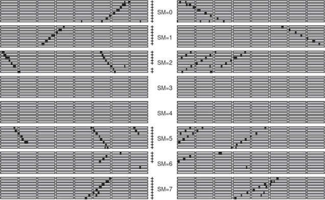
Figure 1. Response of DECOR supermodules to a muon-bundle event.
Download figure:
Standard image High-resolution image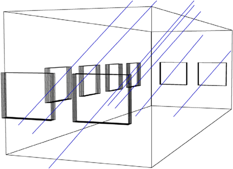
Figure 2. Geometrical reconstruction of the muon-bundle event. The big rectangles are the DECOR supermodules.
Download figure:
Standard image High-resolution imageThe muon bundle is a group of several genetically related muons with quasi-parallel tracks. Muon bundles are generated close to the air-shower core and can reach the detector in a wide range of zenith angles. Moreover, muon bundles retain the direction of the primary particle with good accuracy. Therefore they can be used to study CR anisotropy.
The selection of events is carried out in several steps. First, at the trigger system level, at least three DECOR supermodules must be hit within the time gate of 250 ns. Then, software reconstruction is used to select events by the number of quasi-parallel (within a five-degree cone) tracks. An example of a muon-bundle event detected with the coordinate-tracking detector is shown in Figures 1 and 2. Finally, we select events in which at least three muon tracks with arrival direction zenith angles in the range from 15° to 75° are detected in at least three different SMs.
As mentioned above, the DECOR supermodules have a vertical orientation. This provides a reliable detection of near-horizontal particle tracks. At small zenith angles, the effective area of the detector decreases, and the background from the electron–photon component increases. Therefore, the range of zenith angles from 0° to 15° was excluded from the analysis. On the other hand, the intensity of muon bundles rapidly decreases with the growth of zenith angles. In such conditions, the relative fraction of events with incorrect geometry reconstruction increases at large zenith angles. That is why events with zenith angles greater than 75° were also excluded.
4. Primary Energy Estimation
Estimation of the energy of primary particles was carried out with simulated events using the spectra of the local muon density measured for different zenith angles (Bogdanov et al. 2010). Muon bundles were simulated in the range of zenith angles from 15° to 75° and azimuthal angles from 0° to 90°. The trigger conditions for selecting simulated events were the same as those for real events (see Section 3). The "equivalent time" of a set of simulated events corresponds to about 254 hr of experimental data taking.
To compare the obtained sample of simulated events with the experiment, we used a set of experimental runs with duration of 3459 hr ("live time"). During this time, 830.8 thousand events with arrival directions in the range of zenith angles from 15° to 75° were recorded. As seen in Figure 3, the angular distributions of the simulated and experimental events are in very good agreement. To compare the distributions over the azimuth angle, the experimental data were summarized over four quadrants; the total number of detected events was normalized to the number of simulated ones.
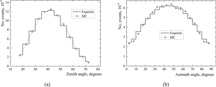
Figure 3. Comparison of distributions in (a) zenith and (b) azimuth angles.
Download figure:
Standard image High-resolution imageTo determine the density of muons in a bundle, the effective area of the detector, which depends on the particle arrival direction, was taken into account. To pass from muon-density distributions to primary-particle energy distributions, it is necessary to use the estimative formula (Bogdanov et al. 2010), which relates the average logarithm of the primary energy to the muon density and zenith angle of the particle arrival direction:

The variable Eest is an intermediate estimator of the primary energy. The distributions of the logarithm of the primary energy estimator (lgEest) obtained using Equation (5) in the simulated events for muon track multiplicities m ≥ 3 and m ≥ 5 are shown in Figure 4. The distribution for the minimal multiplicity of muon tracks m = 3 is rather wide. The long left tail is due to the Poisson fluctuations in the number of tracks in events with low muon densities. With the increase in the threshold number of tracks (transition from m = 3 to m = 5) the distribution becomes narrow, but the statistics decreases by more than 4 times. The numerical characteristics of the distributions of the muon-bundle density D and the logarithm of the primary energy estimator lgEest (mean values and rms deviations) are given in Table 1.
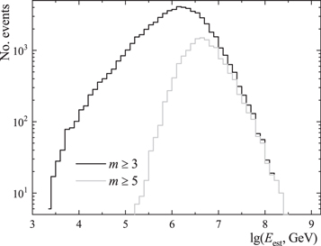
Figure 4. Distributions of the logarithm of the primary energy estimator (Equation (5)) for simulated events.
Download figure:
Standard image High-resolution imageTable 1. Characteristics of the Distributions for Two Samples of Simulated Events
| m | No. ev. | 〈 lg(D, m−2 )〉 | σ(lgD) | 〈 lg(Eest,GeV)〉 | σ(lgEest) | 〈 lgE0,GeV 〉 | σ(lgE0) |
|---|---|---|---|---|---|---|---|
| ≥3 | 64120 | −1.428 ±0.002 | 0.615 | 6.071 ± 0.003 | 0.695 | 6.07±0.10 | 0.80 |
| ≥5 | 14966 | −0.827 ±0.003 | 0.370 | 6.707 ± 0.004 | 0.449 | 6.71±0.10 | 0.60 |
Download table as: ASCIITypeset image
For a correct assessment of the parameters of the distribution in logarithm of the primary energy (lgE0), it should be taken into account that Equation (5) is valid only on the average. The uncertainty in the average value of lgE0 is 0.10 (Bogdanov et al. 2010) and is associated not only with the approximation of Equation (5), but also with the choice of the model of hadronic interaction, the assumption on CR composition, etc.
The rms spread of the logarithm of the primary-particle energies, corresponding to a fixed muon density and a fixed arrival direction, is about 0.4 (Bogdanov et al. 2010). Such spread is associated with the randomness of the EAS core positions relative to the detector location, and its estimate weakly depends on the angle, density, model, and type of primary nuclei. To account for this source of spread, it is necessary to add (in squares) 0.4 to the earlier obtained σ(lgEest). The result of this operation is shown in the last column of Table 1. Thus, two samples of data with minimal track multiplicities (m ≥ 3 and m ≥ 5) correspond to mean logarithmic energies of primary particles of about 1 PeV and 5 PeV, respectively.
In the Galaxy, the gyroradius for protons with such energies is about 1–5 pc or 3–15 light years. It is comparable with the distances to the nearest stars. In this region of space, no particle sources producing particles with such high energies have been discovered yet. So, it is possible to study large-scale anisotropy, while the search for small-scale anisotropy (Aartsen et al. 2016) is rather complicated due to the rapid decrease in intensity with the growth of the primary energy.
5. Experimental Data
The experimental data for the analysis of CR anisotropy were collected in four continuous series of data taking (see Table 2) performed in 2012–2022 at the DECOR detector. The total "live time" of observation was 57 271 hr (∼2 386 days). The "live time" of observation is measured by hardware and is the sum of the time intervals in which the system is ready to accept an event (between the end of processing one event and the appearance of a trigger signal from the next event). The trigger system of the experimental complex combines three installations. One of them is DECOR. The average event counting rate in the trigger system is about 15 events per second. The sampling accuracy of time intervals is 100 ns. Thus, the relative error of measurements of time intervals is 1.5 × 10⁻⁶. The entire period of data taking is divided into four rather long intervals called "series." This division is associated with some minor changes in the configurations of the installations included in the experimental complex. Within each series, the data are segmented into time intervals (called "runs") lasting from 10 to 40 hr. Events with muon bundles were selected according to the conditions described in Section 3. The durations of the series and the numbers of events recorded during each one for two muon-bundle multiplicity thresholds are given in Table 2. With an increase in the threshold from three to five tracks, the number of events decreases by about 3.4 times.
Table 2. Series of Data Taking
| Series | Start | End | No. Events ≥ 3 Tracks | No. Events ≥ 5 Tracks |
|---|---|---|---|---|
| 10 | 2012/5/3 | 2013/3/2 | 1 188 690 | 355 777 |
| 11 | 2013/6/4 | 2015/4/8 | 2 922 316 | 874 525 |
| 12 | 2015/7/16 | 2018/12/25 | 5 878 201 | 1 760 296 |
| 13 | 2019/9/18 | 2022/1/19 | 3 956 759 | 1 166 203 |
| Total | 2012/5/3 | 2022/1/19 | 13 945 966 | 4 156 801 |
Download table as: ASCIITypeset image
In the local coordinate system of the experimental complex, the distribution of events in the zenith angle does not practically change its shape when passing from one threshold to another (Figure 5, left). The distributions in the azimuth angle (Figure 5, right) indicate four preferred directions of detection associated with the azimuthal dependence of the effective area of the DECOR detector.
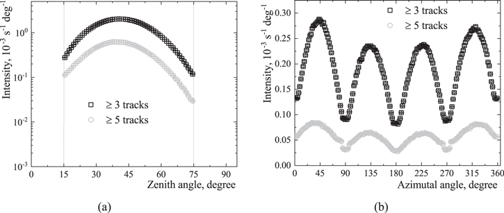
Figure 5. Distributions of events in (a) zenith and (b) azimuth angles.
Download figure:
Standard image High-resolution image6. Correction for the Atmospheric Effect
The muons are generated in the atmosphere mainly through decays of charged pions and kaons, which are components of nuclear cascades initiated by high-energy primary CR particles. This air-shower process develops in the atmosphere, and consequently the parameters of the medium may affect the muon density at the altitude of the detector location. Long-term measurements of muon bundles with the DECOR detector have revealed variations in the intensity of muon bundles (Figure 6). Each point in the plot represents the average rate for one run (from 10 to 40 hr duration) of a series. The blank spaces in Figure 6 separate data of different series. The black curve shows the first annual harmonics of variations. There are both seasonal and short-term variations in the counting rate of the muon bundles.
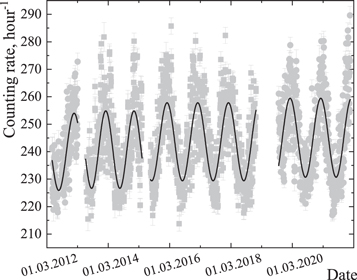
Figure 6. Variations in the counting rate of muon bundles with a selection threshold of three tracks before the correction for atmospheric effects. The black curve shows the first annual harmonics of variations.
Download figure:
Standard image High-resolution imageThe muon-bundle multiplicity is related to the parameters of the lateral distribution function (LDF) of muons at the detection level, which in turn depends on the altitude of their generation in the atmosphere. With the decrease in the altitude of the generation point, the amount of detected events satisfying the selection conditions increases. Based on the analysis of variations in the muon-bundle counting rate, the method for atmospheric-effect compensation (Yurina et al. 2019) was developed in the Experimental Complex NEVOD. This method uses close correlations (correlation coefficient of 0.97) of the muon-bundle counting rate with the altitude of the atmospheric layer with a residual pressure of 500 mbar (H500). The best approximation of the relation between the counting rate and the altitude (H500) is achieved by using a power-law function:

where t is the date and time of measurement, H0 and F0 are the altitude of the atmospheric layer with a residual pressure of 500 mbar and the muon-bundle counting rate averaged over a long period of time, respectively; the power index λ is related to the slope of the spectrum of local muon densities (Yurina et al. 2019). Data on H500 values were taken from the Global Data Assimilation System (GDAS) database (NOAA ARL 2022) for the node closest to the detector (37°N, 56°E) in a one-degree geographic grid. The estimates of the parameters in Equation (6) for each series are presented in Table 3. During more than 9 yr of operation, the configuration of the detector has slightly changed between the series. The changes were mainly concerned with the adjustment of the thresholds for recording pulses from streamer tubes, and with some background conditions. So, the average counting rates in each series are slightly different (see Table 3).
Table 3. Parameters in Equation (6) and Average Counting Rates of Muon Bundles for Each Series of Data Taking
| Series | H0, m | λ | Rate, hr−1 | Corrected Rate, hr−1 |
|---|---|---|---|---|
| 10 | 5524 ± 12 | −1.684 ± 0.034 | 240.9 ± 12.1 | 240.8 ± 3.2 |
| 11 | 5541 ± 9 | −1.688 ± 0.020 | 241.8 ± 13.5 | 240.8 ± 3.2 |
| 12 | 5532 ± 7 | −1.674 ± 0.015 | 243.6 ± 13.9 | 242.9 ± 3.4 |
| 13 | 5515 ± 10 | −1.659 ± 0.021 | 246.3 ± 14.6 | 245.0 ± 3.2 |
Download table as: ASCIITypeset image
The rate errors indicated in the two last columns of Table 3 represent the run-to-run rms spread. The correction for the atmospheric effect resulted in a decrease in the rms spread by about 4 times (Figure 7), and its value (Table 3) almost reached the level of statistical errors of about 1%–2%.
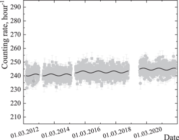
Figure 7. Variations in the counting rate of muon bundles with a selection threshold of three tracks after the correction for atmospheric effects. The black curve shows the first annual harmonics of variations.
Download figure:
Standard image High-resolution imageThe result of correcting for atmospheric effects on the counting rate of muon bundles is shown in Figure 7. The estimated relative amplitudes of the first harmonics of annual and diurnal variations before and after correction for atmospheric effects are given in Table 4.
Table 4. Relative Amplitudes of Annual and Diurnal Variations Before and After the Correction for Atmospheric Effects
| Selection Threshold, Tracks | Annual | Diurnal | ||
|---|---|---|---|---|
| A0, 10−3 | Acorr, 10−3 | A0, 10−3 | Acorr, 10−3 | |
| 3 | 58.34 ± 0.38 | 3.11 ± 0.38 | 1.23 ± 0.38 | 0.31 ± 0.38 |
| 5 | 56.74 ± 0.69 | 1.74 ± 0.70 | 1.23 ± 0.69 | 0.90 ± 0.70 |
Download table as: ASCIITypeset image
The application of the method for atmospheric-effect correction resulted in a significant reduction in the amplitude of the first harmonics of annual variations (by about 20 and 30 times for selection thresholds of three and five tracks, respectively). The diurnal variations are much smaller than the seasonal ones, and are completely suppressed after the introduction of atmospheric correction. Short-term outliers associated with cyclonic activity are also almost completely removed. This fact demonstrates that the seasonal effect and short-term modulations of atmospheric origin were practically eliminated.
7. Estimation of the Expected Number of Events
According to Equation (3), the amplitude of CR flux anisotropy is defined as a relative deviation of the number of recorded events (Nrec) from the amount expected in assumption of an isotropic flux along the selected direction in a given solid angle (Nexp):
To estimate the error (ΔA) of this quantity (A), the following expression is used:

The most convenient way to obtain the expected number of events from a given detection direction is to use the second equatorial coordinate system (Sadler et al. 1974), because this system and the Earth have a common equatorial plane. As an alternative, the galactic coordinate system (Blaauw et al. 1960) may be used. Both systems use two spherical coordinates: latitude and longitude similar to those used on Earth. To present the measurement results we used the HEALPix framework (Gorski et al. 2005) with the Hammer–Aitoff equal-area projection (Calabretta & Greisen 2002) for the pixelization of data on the celestial sphere. The HEALPix grid resolution parameter Nside is set to 64 for all pictures. It corresponds to a cell size of about 2.6 × 10⁻⁴ sr on the celestial sphere.
When estimating the expected number of events, it is important to consider the factors affecting the detection of muon bundles. These factors include: background conditions, design features that affect the detection efficiency for different arrival directions of muon bundles, atmospheric effects, and the inhomogeneity of the time of observation of various parts of the celestial sphere. The estimation method is based on the usage of the available sample of recorded events. To exclude the influence of different background conditions when changing the detector configuration (see Section 5), we processed the data of each series separately and then merged the results. To compensate for the atmospheric effect, we summed the values inverse to the coefficients η(t) in Equation (6) for each cell of the celestial sphere:

where (α, δ) are coordinates of the cell on the celestial sphere, and i is the event number in the given cell. To take the design features into account, we used the so-called "aperture snapshot" (Figure 8). These 2D distributions in the second equatorial and galactic coordinate systems are collected assuming that the sidereal time is constant (for example, it equals zero). In other words, we virtually "stopped" the Earth's rotation around its axis. In this case, the snapshot of all events is the image of the muon-bundle flux multiplied by the aperture of the DECOR detector. In Figure 8, the colors indicate the number of events detected in each cell. Four colored spots on the figure correspond to four highlighted directions in the local coordinate system (see Figure 5). The white spot corresponds to directions with near-vertical zenith angles (θ < 15°). Its center corresponds to the zero zenith angle in the local coordinate system.

Figure 8. Distribution of all events from the sample of 12th series in the celestial sphere for the zero moment of sidereal time plotted in the second equatorial (a) and in the galactic (b) coordinate systems. The red curve represents the Galaxy plane (a) and equatorial plane (b). The red point shows the center of Galaxy (a) and the reference point of the second equatorial coordinate system (b).
Download figure:
Standard image High-resolution imageIn the case of an isotropic flux, all directions are considered as equal, and the number of recorded events in a given solid angle is only related to the duration of measurement. So, to obtain the map of the expected numbers of events, we rotate the aperture snapshot around the world axis together with the Earth and normalize it to the "live time" of observation.
The "live time" of observation is the part of detector operation time after subtraction of the time required for hardware and software processing of events. The distribution of "live time" in the UTC system (solar time) has a dip in the morning period of the day (see Figure 9, left). Its main reason is interruptions of exposition for the detector maintenance. The standard deviation from the mean value of 2386.3 days is approximately 3.4%. The distribution of "live time" within the sidereal day for the entire period of observation is almost uniform (see Figure 9, right), the standard deviation from the average value of 2392.8 days is less than 0.6%.
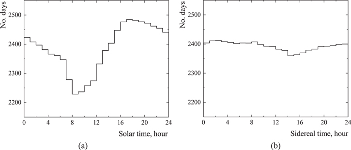
Figure 9. Distribution of "live time" within the solar (left) and sidereal (right) days.
Download figure:
Standard image High-resolution imageAs a result, the distribution of the expected number of events over the celestial sphere has near-axial symmetry (Figure 10) in the second equatorial coordinate system and is uneven over the decl. A significant part of events is detected from the polar region in the second equatorial coordinate system. The expected number of events decreases as it approaches the equatorial plane and disappears in the southern celestial hemisphere. The total decl. range is from −20° to 90°. That is why we cannot observe the area of the celestial sphere where the Galactic center is located (α = 266°, δ = −29°; see Figure 10). The same image plotted in the galactic coordinate system demonstrates that we observe mainly the outer region of the Galaxy, but the data are available over the entire range of galactic longitudes.
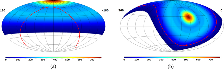
Figure 10. Distribution of the expected number of events with muon bundles from the sample of the 12th series plotted in the second equatorial (left) and in the galactic (right) coordinate systems. The red line represents the Galaxy plane (left) and equatorial plane (right). The red point shows the center of the Galaxy (left) and the reference point of the second equatorial coordinate system (right).
Download figure:
Standard image High-resolution image8. Results and Discussion
Unfortunately, the collected statistics of events still does not allow us to obtain a clear image of the anisotropy of the CR flux on the celestial sphere. The results of data processing for two threshold values of the number of registered tracks are presented in one-dimensional projections on the R.A. and galactic longitude (see Figures 11 and 12). The relation between the minimal number of recorded tracks in the sample and the average logarithm of the primary-particle energy is described in Section 4. To plot the dependences, the entire ranges of R.A. and galactic longitude were divided into 18 bins of 20° degrees each. The data of each series of data taking were analyzed independently from each other. The result for the entire period was obtained as a weighted average, where the weights were determined by the respective statistical errors.

Figure 11. One-dimensional projections of the relative deviations for a selection threshold of three muon tracks on the R.A. (a) and on the galactic longitude (b). The sinusoidal curves represent the best fits.
Download figure:
Standard image High-resolution image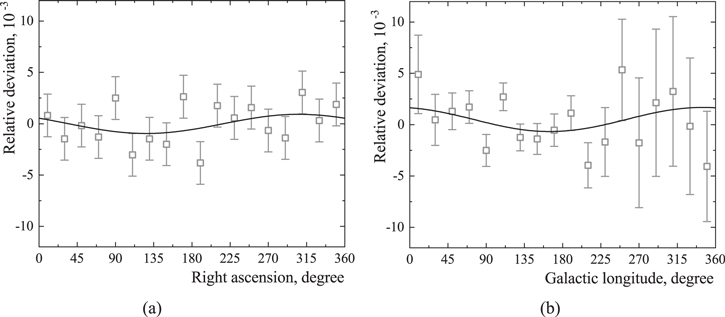
Figure 12. One-dimensional projections of the relative deviations for a threshold of five muon tracks on the R.A. (a) and on the galactic longitude (b). The sinusoidal curves represent the best fits.
Download figure:
Standard image High-resolution imageIn accordance with Equation (4), we approximated these dependences by the function:

The results of fitting are presented in Table 5. In case of the second equatorial coordinate system, parameter b on the left plots can be considered as being equal to zero. In each case, the normalized value of χ2/dof (dof indicates here the number of degrees of freedom) is higher for the hypothesis of an isotropic CR flux. It means that the option of the presence of dipole anisotropy is preferable. The amplitude of the dipole anisotropy corresponds to a significance of about 2.7σ in both the second equatorial and the galactic coordinate systems. The value of the anisotropy phase determined in both coordinate systems agrees with the position of the Galactic center. The deviations of the obtained anisotropy phases in the second equatorial (δφEq) and in the galactic (δφGal) coordinate systems from the direction to the Galactic center (αGC = 266°) are given in Table 5.
Table 5. Parameters of Dipole Anisotropy Approximation
| System | 〈 lg(E,GeV)〉 | a, 10−3 | δφEq/δφGal (degree) | χ2/dof a (dipole) | χ2/dof (Isotropic) |
|---|---|---|---|---|---|
| Second Equat. | 6.07 ± 0.80 | 1.02 ± 0.38 | 10 ± 21 | 22.2/15 | 43.3/15 |
| Second Equat. | 6.71 ± 0.60 | 0.95 ±0.69 | 40 ± 42 | 14.0/15 | 19.8/15 |
| Galactic | 6.07 ± 0.80 | 1.02 ± 0.38 | 2 ± 21 | 12.6/15 | 32.3/15 |
| Galactic | 6.71 ± 0.60 | 1.20 ± 0.69 | −15 ± 33 | 16.1/15 | 24.1/15 |
Note.
a Dof indicates the number of degrees of freedom.Download table as: ASCIITypeset image
Incomplete compensation of the seasonal variations in the muon-bundle intensity after corrections for atmospheric effects (Figure 7; Table 4) might affect the estimates of the dipole anisotropy parameters. Accounting for residual seasonal variations (the third column in Table 4) allowed us to check the influence of this effect on the final fits. As a result, this correction has led to an increase in the estimates of the dipole anisotropy amplitude by (+0.04 ± 0.01) × 10−3; the phases shifted by less than 1°. These values may be considered as systematic uncertainties of the anisotropy parameters. Noteworthy, they are much less than the statistical errors.
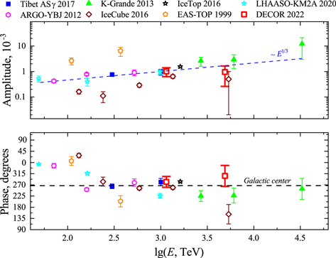
The results of dipole anisotropy measurements in the energy range of primary particles from 0.1 to 30 PeV obtained in different experiments are presented in Figure 13. The anisotropy phase drastically changes near the energy of 0.2 PeV. At energies from few hundred TeV up to about 30 PeV, the anisotropy phase is almost constant. Also, it can be concluded that the phase coincides with the direction to the center of the Galaxy. The dashed line in the upper plot of Figure 13 shows a graph of the dependence of the anisotropy amplitude on the primary energy assumed by diffusion theory (Berezinsky 1990).
Figure 13. Parameters of dipole anisotropy obtained by different experiments.
Download figure:
Standard image High-resolution image
Our results confirm the presence of dipole anisotropy with a significance of 2.7σ. It is possible that with higher statistics we will be able to increase this value. Currently, the parameters of the dipole anisotropy obtained in our research using new methods for anisotropy measurements are consistent with the data of such installations as IceCube (Aartsen et al. 2016) and Tibet-ASγ array (Amenomori et al. 2017), see Figure 13.
9. Conclusions
The research results presented in this paper indicate that muon bundles can be used as a tool for studying the anisotropy of CRs. The methods of data recording and processing developed at the Experimental Complex NEVOD provide suppression and accounting for hampering factors, as well as obtaining reliable results.
It should be mentioned that for the first time the multiplicity of muon bundles is used for the study of the energy dependence of CR anisotropy. Such measurements have been performed for the first time with the coordinate-tracking detector DECOR. Also at the Experimental Complex NEVOD, the new method of correction for atmospheric effects was developed and implemented. The advantage of this method is that the altitude of the atmospheric layer with a residual pressure of 500 mbar is the only parameter necessary for the correction. The results of the performed data analysis demonstrate that the developed method provides almost complete suppressing of the influence of atmospheric effects on the counting rate of muon bundles.
The effective energy of primary particles is related to the density of the detected muon bundles. The average logarithmic energies of primary particles are about 1 PeV and 5 PeV for the selection conditions of at least three and five muon tracks, correspondingly.
The method for estimating the number of events under the assumption of an isotropic flux, which we used in our research, provides an opportunity to consider the design features of the detector and the nonuniformity of its detection efficiency for different arrival directions of muon bundles.
The obtained dipole anisotropy parameters are consistent with the theory of diffuse propagation of CR from the center of the Galaxy.
The work was performed at the Unique Scientific Facility "Experimental Complex NEVOD" with the financial support provided by the Russian Ministry of Science and Higher Education, projects No. 0723-2020-0040 and FSWU-2023-0068.