HOWTO: Multi-scale 3D Gravity and Magnetic Inversion modeling
Alexey Pechnikov
Founder & Developer, InSAR.dev & Geo3D.dev | Geoscience, CS & ML Expert, MSc. Radiophysics
We described mathematics and physics basis for the model before in LinkedIn articles. Also, we provided examples of the 3D models for gas and oil exploration, mineral resources exploration, earthquakes analysis, etc. Below you can find a short introduction with additional links to our articles with geological examples. For some articles we provide live Python3 code in Jupyter notebooks on GitHub:
See also our YouTube channel for animated models:
That’s the reason while we prefer internet publications instead of paper ones where source data unavailable and live data processing pipeline impossible. Let's decide if you prefer a paper article which is not available to check or the LinkedIn publication with all source data and data processing and real user comments.

We base our work on the inverse potential problem solution for gravity and temperature gradient fields to get the 3D density model and 3D heat sources model accordingly. We have our own software product to build the solution (based on numeric finite elements calculation by well-known Saxov-Nygaard method adopted for high accuracy because of high computer power today).


See for details
Inversion of Gravity Field of Deepen Spheres
5 Ways for Inversion of Gravity Field
Often there are no available high-accuracy gravity data and so we need to enhance it by DEM and satellite images data first. That's possible because there is a high correlation between spatial spectrum components of gravity and DEM/ortho photo/satellite image. So we use spectrum components transfer to produce the high-resolution gravity data up to ~1m spatial accuracy. The possible spatial accuracy defining by correlogram analysis.
See for details
Spectral Coherence between Gravity and Bathymetry Grids


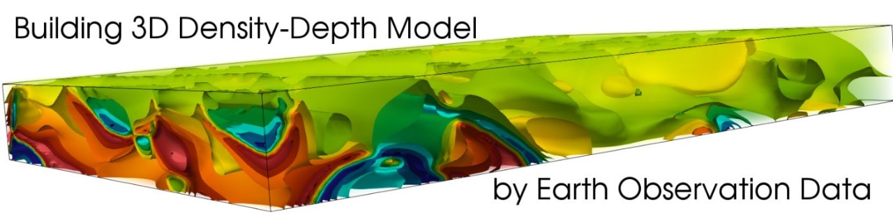
A geological density can be obtained by a fractal dimension index calculation. Our density-depth profile calculation uses as a gravity field as a gravity correlated DEM/ortho photo/satellite images. For the most accurate data processing, the fractal dimension index calculation based on the spatial spectrum and the accuracy controlled by the same correlogram analysis as above.
See for details
The Density-Depth Model by Spectral Fractal Dimension Index

The main point of the 3D Density model ready to use for geological analysis is the right spatial scale. We use band spatial filtering of the source gravity/DEM/etc. data to select only needed spatial band and exclude short scale spectral components (high-frequency) spatial noise and high power long scale spectral components (low-frequency). See for details:
Generalization as Spectral Filtering Effect

The spatial filtering is like to Bouguer and other geophysical reductions which are strong scale-dependent:
What in fact mean Bouguer and Free-Air Gravity Anomalies in terms of spatial spectrum?

For geological explorations a density anomaly model can be much more usable than the original density model. The 3D gradient calculation is the easiest way to produce it. For our analysis we have more complex 3D density anomaly building algorithm. We do not publish the details but usually we provide a comparison between the density anomaly model and the density model gradient. For many cases these two products are similar although the density anomaly model is more detailed.
Recursos Hídricos I Permisos Ambientales I Gestión Ambiental
4yExcellent contribution, thanks